This R script performs a series of tests and analyses on a dataset imported from an Excel file. It first loads the required packages, including readxl for reading Excel files, ggplot2 for data visualization, and nortest for statistical tests. It then sets the working directory and imports the data from the Excel file into a data frame. The script then performs a Shapiro-Wilk test and an Anderson-Darling test to determine whether the data is normally distributed. It plots a histogram and a Q-Q plot of the data to visualize its distribution. Finally, it outputs the test results and determines whether the data is normally distributed at the 5% significance level using conditional statements.
How to Run the Code
The R script performs the following actions:
- Load required packages: The R script loads the required packages, including
readxlfor importing Excel files,ggplot2for data visualization, andnortestfor normality tests. - Set the working directory to the folder where the .xlsx file is located: The R script sets the working directory to the location of the .xlsx file.
- Import the data from the .xlsx file and save it as a data frame: The R script imports the data from the .xlsx file and saves it as a data frame.
- View the first few rows of the data frame to confirm that the data was imported correctly: The R script displays the first few rows of the data frame to check if the data was imported correctly.
- Extract the numeric values from the “Data” column: The R script extracts the numeric values from the “Data” column of the data frame.
- Perform Shapiro-Wilk test for normality: The R script performs the Shapiro-Wilk test for normality using the
shapiro.test()function. - Perform the Anderson-Darling test for normality: The R script performs the Anderson-Darling test for normality using the
ad.test()function. - Plot histogram of the data: The R script plots a histogram of the data using the
hist()function. - Overlay a density plot of the data on top of the histogram: The R script overlays a density plot of the data on top of the histogram using the
lines()function. - Plot a Q-Q plot to visually assess normality of the data: The R script plots a Q-Q plot to visually assess the normality of the data using the
ggplot()function. - Print results of the Shapiro-Wilk test for normality: The R script prints the results of the Shapiro-Wilk test for normality using the
cat()function. - Check if the data is normally distributed at the 5% significance level using the Shapiro-Wilk test: The R script checks if the data is normally distributed at the 5% significance level using the Shapiro-Wilk test and prints the result using the
ifstatement andcat()function. - Print results of the Anderson-Darling test for normality: The R script prints the results of the Anderson-Darling test for normality using the
cat()function. - Check if the data is normally distributed at the 5% significance level using the Anderson-Darling test: The R script checks if the data is normally distributed at the 5% significance level using the Anderson-Darling test and prints the result using the
ifstatement andcat()function.
Overall Code
## Normality Test
#+------+------+
#|  x   |  y   |
#+------+------+
#| 0.25 | 2.46 |
#| 0.26 | 1.99 |
#| 0.15 | 2.13 |
#+------+------+

# Load required packages
library(readxl)
library(ggplot2)
library(nortest)

# Set the working directory to the folder where the .xlsx file is located
input_path <- "C:\\Users\\barbi\\Desktop\\data.xlsx"

significance_level = 0.05

# Import the data from the .xlsx file and save it as a data frame
data <- read_excel(input_path)

# View the first few rows of the data frame to confirm that the data was imported correctly
head(data)

# Extract the numeric values from the "Data" column
data_values <- data$Data

# Perform Shapiro-Wilk test
result_sw <- shapiro.test(data_values)


# Perform the Anderson-Darling test
result_ad <- ad.test(data_values)


# Plot histogram
hist(data_values, freq = FALSE, main = "Normal Distribucion Plot", xlab = "Data", ylab = "Density", col = "gray")
lines(density(data_values), col = "blue", lwd = 2)


Sys.sleep(3)


# Plot Q-Q plot
df <- data.frame(x = data_values)

ggplot(df, aes(sample = x)) +
  stat_qq() +
  stat_qq_line()


# Results for Shapiro-Wilk test
cat("Shapiro-Wilk test:", result_sw$statistic, "\n")
cat("p-value:", result_sw$p.value, "\n")
9
# Check if the data is normally distributed at the 5% significance level
if (result_sw$p.value < significance_level) {
  cat("The data is not normally distributed.\n")
} else {
  cat("The data is normally distributed.\n")
}


# Results for Anderson-Darling
cat("Anderson-Darling test statistic:", result_ad$statistic, "\n")
cat("p-value:", result_ad$p.value, "\n")

# Check if the data is normally distributed at the 5% significance level
if (result_ad$p.value < 0.05) {
  cat("The data is not normally distributed.\n")
} else {
  cat("The data is normally distributed.\n")
}
References:
- Wickham, Hadley; Bryan, J. Readxl: Read Excel Files. 2019. https://cran.r-project.org/package=readxl.
- Wickham, H. ggplot2: Elegant Graphics for Data Analysis. 2016. https://ggplot2.tidyverse.org.

Classifies, quantifies, and explores data using spectroscopy techniques coupled with chemometric routines.