This R script conducts a one-way ANOVA test to determine if there is a significant difference between the means of multiple groups. The script first reads in data from an Excel file, combines the data for all groups into a single data frame, and computes summary statistics for each group. It then performs an ANOVA test using the ‘aov’ function and extracts the ANOVA table and results. The script concludes by printing the results and deciding whether to reject or fail to reject the null hypothesis based on the p-value and F-statistic. Finally, the script creates a new Excel workbook and writes the original data, ANOVA results, conclusion, and summary statistics to different worksheets within the workbook.
How to Run the Code
Before using the R script, you need to ensure that you have the following:
- An Excel file with data to be analyzed. The data should be organized such that the samples are in rows, and the groups are in columns.
- R and RStudio installed on your computer.
- The following R packages installed: tibble, readxl, stats, openxlsx, tidyr, and broom.
Once you have these prerequisites, follow the steps below to use the script:
Step 1: Open RStudio on your computer and create a new script file.
Step 2: Copy and paste the R script into the new script file.
Step 3: Fill in the following parameters at the beginning of the script:
- input_path: The file path to your input Excel file containing the data to be analyzed.
- output_path: The file path where you want to save the output Excel file containing the ANOVA results.
- significance_level: The significance level to be used in the ANOVA test.
- repetitions: The number of repetitions for each group.
Step 4: Load the required packages by running the following code in RStudio:
library(tibble)

library(readxl)

library(stats)

library(openxlsx)

library(tidyr)

library(broom)
library(multcomp)Step 5: Read in the data from the Excel file by running the following code:
my_data <- read_excel(input_path)

my_data <- as.data.frame(my_data)
Step 6: Combine the data for all groups into a single data frame by running the following code:
group_dfs <- lapply(1:repetitions, function(x) {

group_data <- my_data[, x]

data.frame(Group = rep(x, nrow(my_data)), Value = group_data, check.names = FALSE)

})

combined_data <- do.call(rbind, group_dfs)
Here, we use the lapply() function to iterate over the columns in my_data and create a list of data frames, each containing the data for one group. We then combine the data frames using do.call(rbind, group_dfs) to create a single data frame with all the data.
Step 7: Compute the summary statistics by running the following code:
count <- tapply(combined_data$Value, combined_data$Group, length)

sum <- tapply(combined_data$Value, combined_data$Group, sum)

mean <- tapply(combined_data$Value, combined_data$Group, mean)

var <- tapply(combined_data$Value, combined_data$Group, var)

summary_statistics <- data.frame(Group = 1:repetitions, Count = count, Sum = sum, Average = mean, Variance = var)
Here, we use the tapply() function to compute the count, sum, mean, and variance for each group, and then combine the results into a data frame.
Step 8: Convert the data frame to a tibble and convert it from wide to long format by running the following code:
my_data <- as_tibble(my_data)

my_data <- pivot_longer(my_data, cols = everything(), names_to = "labels", values_to = "factor", names_prefix = "Var", values_drop_na = TRUE)

my_data <- my_data[order(my_data$labels),]
Here, we use the as_tibble() function to convert my_data to a tibble, and then use the pivot_longer() function to convert it from wide to long format. We also use the order() function to sort the data by the labels column.
Step 9: Perform the ANOVA test by running
Overall Code
## ONE WAY (1 FACTOR) ANOVA
# Place data in a .xlsx file
# Samples in rows and groups in columns
#+---------+---------+---------+---------+
#| Group 1 | Group 2 | Group 3 | Group 4 |
#+---------+---------+---------+---------+
#| 1.006 | 0.998 | 0.991 | 1.005 |
#| 0.996 | 1.006 | 0.987 | 1.002 |
#| 0.998 | 1.000 | 0.997 | 0.994 |
#+---------+---------+---------+---------+
# Load required packages
library(tibble)
library(readxl)
library(stats)
library(openxlsx)
library(tidyr)
library(broom)
library(multcomp)
# Fill these
input_path <- "C:\\Users\\barbi\\Desktop\\data_one-f-anova.xlsx"
output_path <- "C:\\Users\\barbi\\Desktop\\anova_output.xlsx"
significance_level <- 0.05
repetitions <- 10
# Read in data from Excel file
my_data <- read_excel(input_path)
my_data <- as.data.frame(my_data)
#########################################################################################
#PART 01: PREPARING DATA FOR ANOVA
#########################################################################################
##Modifying data to have the desired format for ANOVA
# Combine data for all n groups (repetitions) into a single data frame
group_dfs <- lapply(1:repetitions, function(x) {
group_data <- my_data[, x]
data.frame(Group = rep(x, nrow(my_data)), Value = group_data, check.names = FALSE)
})
# Combine the dataframes using rbind
combined_data <- do.call(rbind, group_dfs)
colnames(combined_data)[1] <- "Factor"
colnames(combined_data)[2] <- "Response"
# Compute summary statistics
count <- tapply(combined_data$Response, combined_data$Factor, length)
sum <- tapply(combined_data$Response, combined_data$Factor, sum)
mean <- tapply(combined_data$Response, combined_data$Factor, mean)
var <- tapply(combined_data$Response, combined_data$Factor, var)
summary_statistics <- data.frame(Group = 1:10, Count = count, Sum = sum, Average = mean, Variance = var)
summary_statistics
# Convert the data frame to a tibble
my_data <- as_tibble(my_data)
# Convert the data frame from wide to long format
my_data <- pivot_longer(my_data, cols = everything(), names_to = "labels", values_to = "factor", names_prefix = "Var", values_drop_na = TRUE)
my_data <- my_data[order(my_data$labels),]
# View the original column names
colnames(my_data)
# Change the column names using the `names()` function
names(my_data) <- c("Factor", "Response")
# Define the 'Factor' column as a factor
my_data$Factor <- factor(my_data$Factor)
##PERFORMING ANOVA
aov.out <- aov(Response ~ Factor, data = my_data)
#########################################################################################
#PART 02: EFFECT AND GENERAL RESULTS
#########################################################################################
# Extract ANOVA table
anova_table <- as.data.frame(anova(aov.out))
# Extract the results from the ANOVA test
DF_labels = anova_table$Df[1]
DF_residuals = anova_table$Df[2]
SS_labels = anova_table$`Sum Sq`[1]
SS_residuals = anova_table$`Sum Sq`[2]
MS_labels = anova_table$`Mean Sq`[1]
MS_residuals = anova_table$`Mean Sq`[2]
F_statistic <- anova_table$F[1]
F_critical_value <- qf(0.95, length(unique(combined_data$Factor))-1, aov.out$df.resid)
p_value <- anova_table$"Pr(>F)"[1]
# Calculate Eta-Squared
SS_total <- sum((my_data$Response - mean(my_data$Response))^2)
SS_factor <- sum((tapply(my_data$Response, my_data$Factor, mean) - mean(my_data$Response))^2)
Eta_squared <- SS_factor / SS_total
cat("\nEta-squared = ", round(Eta_squared, 3), "\n")
#Calculate Omega-Squared
omega_squared <- (SS_total - (anova_table$Df[1] * MS_residuals)) / (SS_total + MS_residuals)
cat("\nOmega-squared = ", round(omega_squared, 3), "\n")
#Post-hoc: Bonferroni Correction
bonferroni_corr <- p.adjust(p_value, method = "bonferroni")
# Create a data frame with ANOVA results
anova_results <- data.frame(
DF_Between = DF_labels,
DF_Within = DF_residuals,
SS_Between = SS_labels,
SS_Within = SS_residuals,
MS_Between = MS_labels,
MS_Within = MS_residuals,
F_statistic = F_statistic,
F_critical_value = F_critical_value,
p_value = p_value,
Eta_squared = Eta_squared,
bonferroni_corr = bonferroni_corr,
Omega_squared = omega_squared,
alpha = significance_level)
anova_results
#########################################################################################
#PART 03: POST HOC TESTS
#########################################################################################
#Post-hoc: Bonferroni Correction
cat("\nBonferroni-Correction = ", round(bonferroni_corr, 3), "\n")
#Post-hoc: Tukey's HSD
tukey <- TukeyHSD(aov.out)
tukey_table <- tidy(tukey)
tukey_df <- as.data.frame(tukey_table)
#Post-hoc: Scheffe's test
mc <- glht(aov.out, linfct = mcp(Factor = "Tukey"))
summary(mc)
mc_summary <- summary(mc)
scheffe_sum <- tidy(mc_summary)
head(scheffe_sum)
#Pair of groups are significantly different from each other if the adjusted p-value < 0.05.
#########################################################################################
#PART 04: CONCLUSIONS
#########################################################################################
# Function to generate conclusions based on parameters and characteristics
generate_conclusions <- function(p_value, F_statistic, Eta_squared, omega_squared, bonferroni_corr) {
conclusions <- data.frame(Variable = character(), Conclusions = character(), stringsAsFactors = FALSE)
# p-value conclusion
if (p_value < significance_level) {
conclusions <- rbind(conclusions, data.frame(Variable = "p-value < alpha.Reject the null hypothesis.There is significant evidence to support the alternative hypothesis.Hence, at least one group mean is different from the others."))
} else {
conclusions <- rbind(conclusions, data.frame(Variable = "p-value > alpha.Fail to reject the null hypothesis.There is not enough evidence to support the alternative hypothesis.Hence, there is no significant evidence to determine that at least one group mean is different from the others."))
}
# F-statistic conclusion
if (F_statistic < F_critical_value) {
conclusions <- rbind(conclusions, data.frame(Variable = "F < Fcrit.Fail to reject the null hypothesis.There is not enough evidence to support the alternative hypothesis.Hence, there is no significant evidence to determine that at least one group mean is different from the others."))
} else {
conclusions <- rbind(conclusions, data.frame(Variable = "F > Fcrit.Reject the null hypothesis.There is significant evidence to support the alternative hypothesis.Hence, at least one group mean is different from the others.."))
}
# Effect Size: Eta-squared conclusion
if (Eta_squared < 0.01) {
conclusions <- rbind(conclusions, data.frame(Variable = "Eta-squared < 0.01.The differences between groups are very small, and may not be practically significant."))
} else if (Eta_squared < 0.06) {
conclusions <- rbind(conclusions, data.frame(Variable = "Eta_squared < 0.06.The differences between groups are moderate, and may be practically significant depending on the context."))
} else {
conclusions <- rbind(conclusions, data.frame(Variable = "Eta_squared > 0.06.The differences between groups are large, and are likely to be practically significant."))
}
# Effect Size: Omega-squared conclusion
if (omega_squared < 0.01) {
conclusions <- rbind(conclusions, data.frame(Variable = "omega-squared < 0.01.The differences between groups are very small and may not be practically significant."))
} else if (omega_squared < 0.06) {
conclusions <- rbind(conclusions, data.frame(Variable = "omega_squared < 0.06.The differences between groups are moderate and may be practically significant depending on the context."))
} else {
conclusions <- rbind(conclusions, data.frame(Variable = "omega_squared > 0.06.The differences between groups are large and are likely to be practically significant."))
}
return(conclusions)
}
# Generate conclusions based on parameters and characteristics
conclusions_df <- generate_conclusions(p_value, F_statistic, Eta_squared, omega_squared, bonferroni_corr)
# Print the conclusions data frame
print(conclusions_df)
# Post-hoc: Bonferroni Correction conclusion
if (any(bonferroni_corr < significance_level)) {
significant_comparisons <- which(bonferroni_corr < significance_level)
paste("There are significant differences between group", significant_comparisons)
} else {
"There are no significant differences between the groups"
}
if (bonferroni_corr < significance_level) {
b_result_text <- "b < alpha.There are significant differences between group\n"
} else {
b_result_text <- "b > alpha.There are no significant differences between the groups\n"
}
#########################################################################################
#PART 05: SAVING RESULTS
#########################################################################################
# Create a new workbook and add worksheets
wb <- createWorkbook()
addWorksheet(wb, "Original Data")
addWorksheet(wb, "ANOVA Results")
addWorksheet(wb, "CONCLUSIONS")
addWorksheet(wb, "b CONCLUSION")
addWorksheet(wb, "S CONCLUSION")
addWorksheet(wb, "Post-Hoc Tukey")
addWorksheet(wb, "Group Statistics")
# Write original data and ANOVA results to worksheets
writeData(wb, "Original Data", my_data)
writeData(wb, "ANOVA Results", anova_results, startCol = 1, startRow = 1)
writeData(wb, "CONCLUSIONS", conclusions_df)
writeData(wb, "b CONCLUSION", b_result_text)
writeData(wb, "S CONCLUSION", scheffe_sum)
writeData(wb, "Post-Hoc Tukey", tukey_df)
writeData(wb, "Group Statistics", summary_statistics)
# Save the workbook
saveWorkbook(wb, output_path)
References:
- Wickham, Hadley; Bryan, J. Readxl: Read Excel Files. 2019. https://cran.r-project.org/package=readxl.
- Wickham, H. ggplot2: Elegant Graphics for Data Analysis. 2016. https://ggplot2.tidyverse.org.

Classifies, quantifies, and explores data using spectroscopy techniques coupled with chemometric routines.