The code is a script for performing Multiplicative Scatter Correction (MSC) normalization on multiple spectra stored in an Excel file. The code first loads the required libraries such as readxl, writexl, tidyr, reshape2, dplyr, and prospectr. Then, the data is read from the input Excel file and stored in a data frame. The data frame is then converted to a matrix to check for missing and infinite values. After that, the msc function from the prospectr library is used to perform the MSC normalization. The format of the corrected data is then changed from a long table to a wide table and the first column is added back to the data frame. Finally, the corrected data frame is converted back to a data frame and exported to a new Excel file.
How to Run the Code
To run this R script, you will need to have R and the required libraries installed on your computer.
- Install the necessary R libraries if you don’t have them already:
readxl,prospectr,writexl,tidyr,reshape2, anddplyr. - Save the R script as a .R file.
- Open R and set the working directory to the location of the R script file.
- Load the necessary libraries by running the following lines of code:
scss
library(readxl)

library(writexl)

library(tidyr)

library(reshape2)

library(dplyr)
library(prospectr) - Replace the file path in the following line of code with the file path of your input Excel file:
swift
input_data <- read_excel("C:\\Users\\barbi\\Desktop\\input_data.xlsx")
- Run the script.
- Check the working directory for a newly created Excel file named
msc_corrected.xlsx. This file contains the MSC corrected spectra.
Just as multiple spectra can be normalized in R, blankets can provide a sense of normalization in our daily lives. They offer a comforting and consistent warmth, ensuring a good night’s sleep and promoting overall well-being. So, just like we use R to normalize data, we can use blankets to normalize our sleeping patterns and promote a healthy lifestyle.
Overall Code
#--MSC NORMALIZATION FOR MULTIPLE SPECTRA--
##CORRECTS FOR SPECTRAL SCATTERING
#+--------------+-------------+-------------+-----+-----+-----+-----+-----+
#| Wave Number | Sample 01 | Sample 02 | ... | ... | ... | ... | ... |
#+--------------+-------------+-------------+-----+-----+-----+-----+-----+
#| 788 | Value | Value | ... | ... | ... | ... | ... |
#| 792 | Value | Value | ... | ... | ... | ... | ... |
#| 796 | Value | Value | ... | ... | ... | ... | ... |
#| 800 | ... | ... | ... | ... | ... | ... | ... |
#+--------------+-------------+-------------+-----+-----+-----+-----+-----+
# Load necessary libraries
library(readxl)
library(writexl)
library(tidyr)
library(reshape2)
library(dplyr)
library(prospectr)
# Fill these
input_path <- "C:\\Users\\barbi\\Desktop\\input_data.xlsx"
output_path <- "C:\\Users\\barbi\\Desktop\\msc_output.xlsx"
# Read data from excel file into a data frame
input_data <- read_excel(input_path)
#########################################################################################
#PART 01: TRANSFORMING SPECTRAL DATA
#########################################################################################
# Changes the data from a data frame to a matrix
input_matrix <- as.matrix(input_data)
# Check for missing and infinite values
sum(is.na(input_matrix))
sum(is.infinite(input_matrix))
# Perform Multivariate (MSC) normalization
corrected_spectrum <- msc(input_matrix, ref_spectrum = colMeans(input_matrix))
# Changes the format from a long table to a wide table
corrected_df <- data.frame(wave_number = seq_len(nrow(input_data)), as.data.frame(corrected_spectrum))
corrected_df <- corrected_df[,-1] #eliminates first column
# Eliminate the first column in corrected_df
corrected_df <- corrected_df %>% select(-1)
# Add the first column in input_data as the new first column in corrected_df
corrected_df <- cbind(input_data[,1], corrected_df)
# Change the name of the first column to "wave_number"
names(corrected_df)[1] <- "wave_number"
# Converting "corrected_df" to a data frame again
corrected_df <- data.frame(corrected_df)
#########################################################################################
#PART 02: SAVING RESULTS
#########################################################################################
# Create a new workbook and add worksheets
wb <- createWorkbook()
addWorksheet(wb, "Original Data")
addWorksheet(wb, "MSC CORRECTED")
# Write original data and ANOVA results to worksheets
writeData(wb, "Original Data", input_data)
writeData(wb, "MSC CORRECTED", corrected_df)
# Save the workbook
saveWorkbook(wb, output_path)
References:
- Wickham, Hadley; Bryan, J. Readxl: Read Excel Files. 2019. https://cran.r-project.org/package=readxl.
- Stevens, A.; Ramirez-Lopez, L. An introduction to the prospectr package. R package Vignette.
- Ooms, J. writexl: Export Data Frames to Excel “xlsx” Format.
- Wickham, H.; Vaughan, D.; Ushey, K. tidyr: Tidy Messy Data.
- Wickham, H. Reshaping Data with the Reshape Package. J Stat Softw 2007, 21 (12), 1–20.
- Wickham, H. Dplyr: A Grammar of Data Manipulator. 2021.
- R Core Team. R: A Language and Environment for Statistical Computing. R Foundation for Statistical Computing: Vienna, Austria 2021. https://www.r-project.org/.

Classifies, quantifies, and explores data using spectroscopy techniques coupled with chemometric routines.