The provided R script performs variogram analysis. Variogram analysis is a technique used in geostatistics to analyze the spatial dependence or correlation of a variable across a geographic area. The script is divided into three parts.
In Part 01, the necessary packages are loaded, such as “gstat,” “sp,” “tibble,” “readxl,” “stats,” “openxlsx,” “tidyr,” “ggplot2,” “writexl,” “broom,” “multcomp,” and “gridExtra.” The input and output file paths are specified. The data is imported from an Excel file and converted into a spatial points data frame (SPDF). The script then generates the experimental variogram by fitting a variogram model to the data and calculates the distance and gamma values. Finally, the experimental variogram is plotted using ggplot2.
In Part 02, the script focuses on improving the variogram models. The user is instructed to change the parameters (sill, nugget, and range) to improve the models’ fit to the experimental variogram. The script generates variogram models using different models (spherical, exponential, linear, and Gaussian) and computes variogram values for each model. Root Mean Square Error (RMSE) is calculated to assess the fit of each model. The variogram models, along with the initial fit and the current fit, are plotted using ggplot2.
In Part 03, the script saves the data and results. It creates a new Excel workbook and adds worksheets for the original data, experimental variogram, model variograms, parameters, and conclusions. The results, including the variogram values for each model, parameter values, and conclusions based on the parameters and characteristics, are written to the respective worksheets. Finally, the workbook is saved to the specified output path.
How to Run the Code
Before using the R script, you need to ensure that you have the following:
- An Excel file (*.xlsx) with data to be analyzed. The data should be organized such that the samples are in rows, and the groups are in columns.
- Data is comprised of 3 columns: Col. 01 = latitude (x coordinates), Col. 02 = longitude (y coordinates), Col. 03 = z (desired measurement per point in the space).
- R and RStudio installed on your computer.
- The following R packages installed: gstat, sp, tibble, readxl, stats, openxlsx, tidyr, ggplot2, writexl, broom, multcomp, and gridExtra. Use the “install.packages(“package_name”)” function to install the packages.
Once you have these prerequisites, follow the steps below to use the script:
Step 1: Prepare the Data Ensure that your data is in the required format. The data should be an Excel file (.xlsx) with three columns: latitude (x coordinates), longitude (y coordinates), and the desired measurement per point in space (z). Modify the input and output file paths in the script to match the location of your data and where you want to save the output.
Step 2: Run Part 01 – Developing Experimental Variogram Copy and paste Part 01 of the script into your R environment. This section loads the required packages and sets the input and output file paths. It then imports the data from the specified Excel file and converts it into a spatial points data frame (SPDF). The experimental variogram is generated by fitting a variogram model to the data and extracting the distance and gamma values. Finally, the script plots the experimental variogram using ggplot2. Run Part 01 by executing the code.
Step 3: Analyze Initial Fit After running Part 01, the initial fit of the variogram models will be plotted. The plot will show the experimental variogram as blue points and the variogram models (spherical, exponential, linear, and Gaussian) as lines in different colors. The RMSE values for each model will also be displayed. Analyze the initial fit and note the RMSE values for each model.
Step 4: Improve Variogram Models (Part 02) Copy and paste Part 02 of the script into your R environment. This section focuses on improving the variogram models based on the initial fit. You need to change the parameters (sill, nugget, and range) to refine the models’ fit to the experimental variogram. Modify the values of sill, nugget, and range in the script and run Part 02. Repeat this step iteratively, adjusting the parameter values until you achieve a satisfactory fit.
Step 5: Compare Initial and Current Fit After running Part 02, the current fit of the variogram models will be plotted alongside the initial fit. The two plots will be displayed side by side for comparison. Analyze the current fit and compare it to the initial fit. Note any improvements or changes in the RMSE values.
Step 6: Generate Conclusions At this point, you have refined the variogram models and obtained the final fit. Copy and paste the conclusion generation code from Part 02. This code generates conclusions based on the parameter values and characteristics of the models. Run the conclusion generation code to obtain the conclusions as a data frame.
Step 7: Save Data and Results (Part 03) Copy and paste Part 03 of the script into your R environment. This section saves the data and results to an Excel workbook. It creates a new workbook and adds worksheets for the original data, experimental variogram, model variograms, parameters, and conclusions. The data and results are written to their respective worksheets. Modify the output path in
the script to specify where you want to save the Excel workbook. Run Part 03 to save the data and results.
Step 9: Analyze Saved Results Open the saved Excel workbook and review the worksheets. The original data, experimental variogram, model variograms, parameters, and conclusions will be available for analysis. Use this information for further analysis or reporting as needed.
Overall Code
##VARIOGRAM ANALYSIS
##Data needs to be comprised of 3 columns
##Column 1 = latitude (x coordinates), Column 2 = longitude (y coordinates),
##Column 3 = z (desired measurement per point in the space).
##File needs to be .xlsx. Install all the packages below before running using
##install.packages("package_name"), replace "package_name" with the package name.
#+-----------+------------+-----+
#| Latitude | Longitude | z |
#+-----------+------------+-----+
#| ... | ... | ... |
#| ... | ... | ... |
#| ... | ... | ... |
#+-----------+------------+-----+
##################################################################################
DO NOT COPY/PASTE THE ENTIRE CODE, IT IS DIVIDED IN 3 PARTS.
COPY/PASTE PART 01 FIRST, you will see when the other part appears.
##################################################################################
PART 01: DEVELOPING EXPERIMENTAL VARIOGRAM
##################################################################################
## Load the required packages
library(gstat)
library(sp)
library(tibble)
library(readxl)
library(stats)
library(openxlsx)
library(tidyr)
library(ggplot2)
library(writexl)
library(broom)
library(multcomp)
library(gridExtra)
##FILL THESE
input_path <- "C:\\Users\\barbi\\Desktop\\variogram-example.xlsx"
output_path <- "C:\\Users\\barbi\\Desktop\\variogram_output.xlsx"
##IMPORTING DATA
data <- read_excel(input_path)
# Convert data to a spatial points data frame (SPDF)
coordinates(data) <- ~longitude + latitude
##GENERATING EXPERIMENTAL VARIOGRAM
# Create experimental variogram
exp_variogram <- variogram(z ~ 1, data)
# Extract distance and gamma values
exp_variogram_data <- data.frame(distance = exp_variogram$dist, gamma = exp_variogram$gamma)
# Plot the experimental variogram
ggplot(exp_variogram_data, aes(x = distance, y = gamma)) +
geom_point() +
geom_line() +
labs(x = "Lag (h)", y = "Semivariance") +
theme_minimal()
sill <- max(exp_variogram_data$gamma)
nugget <- exp_variogram_data$gamma[1]
range <- exp_variogram_data$distance[which.max(exp_variogram_data$gamma)]
cat("Sill: ", sill, "\n")
cat("Nugget: ", nugget, "\n")
cat("Range: ", range, "\n")
##GENERATING VARIOGRAM MODELS
# Generate variogram models
spherical_model <- vgm(psill = sill, model = "Sph", range = range, nugget = nugget)
exponential_model <- vgm(psill = sill, model = "Exp", range = range, nugget = nugget)
linear_model <- vgm(psill = sill, model = "Lin", range = range, nugget = nugget)
gaussian_model <- vgm(psill = sill, model = "Gau", range = range, nugget = nugget)
# Compute variogram values for the models
spherical_variogram <- variogramLine(spherical_model, maxdist = max(exp_variogram_data$distance))
exponential_variogram <- variogramLine(exponential_model, maxdist = max(exp_variogram_data$distance))
linear_variogram <- variogramLine(linear_model, maxdist = max(exp_variogram_data$distance))
gaussian_variogram <- variogramLine(gaussian_model, maxdist = max(exp_variogram_data$distance))
# Calculate RMSE for each model
spherical_rmse <- sqrt(mean((spherical_variogram$gamma - exp_variogram_data$gamma)^2))
exponential_rmse <- sqrt(mean((exponential_variogram$gamma - exp_variogram_data$gamma)^2))
linear_rmse <- sqrt(mean((linear_variogram$gamma - exp_variogram_data$gamma)^2))
gaussian_rmse <- sqrt(mean((gaussian_variogram$gamma - exp_variogram_data$gamma)^2))
# Create a data frame for the legend labels
legend_df <- data.frame(model = c("Spherical", "Exponential", "Linear", "Gaussian"),
color = c("red", "green", "purple", "orange"))
# Plot the variograms
initial_fit <- ggplot(exp_variogram_data, aes(x = distance, y = gamma)) +
geom_point(color = "blue") +
geom_line(data = spherical_variogram, aes(x = dist, y = gamma), color = "red") +
geom_line(data = exponential_variogram, aes(x = dist, y = gamma), color = "green") +
geom_line(data = linear_variogram, aes(x = dist, y = gamma), color = "purple") +
geom_line(data = gaussian_variogram, aes(x = dist, y = gamma), color = "orange") +
labs(x = "Lag (h)", y = "Semivariance", title = "Variogram Models") +
scale_color_manual(values = legend_df$color, labels = legend_df$model) +
annotate("text", x = 10, y = max(exp_variogram$gamma), label = paste0("Spherical RMSE: ", round(spherical_rmse, 2))) +
annotate("text", x = 10, y = max(exp_variogram$gamma) - 0.5, label = paste0("Exponential RMSE: ", round(exponential_rmse, 2))) +
annotate("text", x = 10, y = max(exp_variogram$gamma) - 1, label = paste0("Linear RMSE: ", round(linear_rmse, 2))) +
annotate("text", x = 10, y = max(exp_variogram$gamma) - 1.5, label = paste0("Gaussian RMSE: ", round(gaussian_rmse, 2))) +
theme_minimal()
initial_fit
#########################################################################################
PART 02: IMPROVING VARIOGRAM MODELS
#RUN THIS PART **AFTER** YOU DO PART 01
#########################################################################################
#Change the sill, nugget, and range to improve the models.
#Range changes when the line goes from increase to stabilizing horizintally
#Sill brings the increase-stabilizing part of the line upwards or downwards
#Nugget brings the whole line downwards or upwards
#CHANGE TO IMPROVE MODELS
sill <- 9.5
nugget <- 0.035
range <- 35
#Copy/Paste this part and change parameters until the variogram model fits
#the experimental variogram best.
## GENERATING VARIOGRAM MODELS
# Generate variogram models
spherical_model <- vgm(psill = sill, model = "Sph", range = range, nugget = nugget)
exponential_model <- vgm(psill = sill, model = "Exp", range = range, nugget = nugget)
linear_model <- vgm(psill = sill, model = "Lin", range = range, nugget = nugget)
gaussian_model <- vgm(psill = sill, model = "Gau", range = range, nugget = nugget)
# Compute variogram values for the models
spherical_variogram <- variogramLine(spherical_model, maxdist = max(exp_variogram_data$distance))
exponential_variogram <- variogramLine(exponential_model, maxdist = max(exp_variogram_data$distance))
linear_variogram <- variogramLine(linear_model, maxdist = max(exp_variogram_data$distance))
gaussian_variogram <- variogramLine(gaussian_model, maxdist = max(exp_variogram_data$distance))
# Create a data frame for the legend labels
legend_df <- data.frame(model = c("Spherical", "Exponential", "Linear", "Gaussian"),
color = c("red", "green", "purple", "orange"))
# Plot the variograms
current_fit <- ggplot(exp_variogram_data, aes(x = distance, y = gamma)) +
geom_point(color = "blue") +
geom_line(data = spherical_variogram, aes(x = dist, y = gamma), color = "red") +
geom_line(data = exponential_variogram, aes(x = dist, y = gamma), color = "green") +
geom_line(data = linear_variogram, aes(x = dist, y = gamma), color = "purple") +
geom_line(data = gaussian_variogram, aes(x = dist, y = gamma), color = "orange") +
labs(x = "Lag (h)", y = "Semivariance", title = "Variogram Models") +
scale_color_manual(values = legend_df$color, labels = legend_df$model) +
theme_minimal()
current_fit
#View the initial fit and current_fit
grid.arrange(initial_fit, current_fit, ncol = 2)
##CONCLUSIONS
# Function to generate conclusions based on parameters and characteristics
generate_conclusions <- function(sill, nugget, range) {
conclusions <- data.frame(Conclusions = character(), stringsAsFactors = FALSE)
# Conclusions based on sill, nugget, and range parameters
if (sill > 0) {
conclusions <- rbind(conclusions, data.frame(Conclusions = "s > 0. The data exhibits variability."))
} else {
conclusions <- rbind(conclusions, data.frame(Conclusions = "s < 0. The data has no variability."))
}
if (nugget > 0) {
conclusions <- rbind(conclusions, data.frame(Conclusions = "c > 0. There is a spatial variation at very short distances or measurement errors."))
}
if (range > 0) {
conclusions <- rbind(conclusions, data.frame(Conclusions = "r > 0. The spatial correlation extends up to a certain range."))
} else {
conclusions <- rbind(conclusions, data.frame(Conclusions = "r < 0. The data does not exhibit spatial correlation."))
}
# Additional conclusions based on characteristics
if (sill > 0 && range > 0) {
conclusions <- rbind(conclusions, data.frame(Conclusions = "s > 0 and r > 0. The data shows spatial heterogeneity and dependency."))
} else {
conclusions <- rbind(conclusions, data.frame(Conclusions = "s < 0 and r < 0. The data does not show clear spatial heterogeneity or dependency."))
}
if (sill > 0 && range == 0) {
conclusions <- rbind(conclusions, data.frame(Conclusions = "s > 0 and r = 0. The data exhibits spatial clustering."))
}
return(conclusions)
}
# Generate conclusions based on parameters and characteristics
conclusions_df <- generate_conclusions(sill, nugget, range)
# Print the conclusions data frame
print(conclusions_df)
##########################################################################################
PART 03: SAVING RESULTS
#RUN THIS PART **AFTER** YOU DO PART 02
##########################################################################################
##SAVE DATA AND RESULTS
# Create a new workbook and add worksheets
wb <- createWorkbook()
addWorksheet(wb, "Original Data")
addWorksheet(wb, "Experimental Variogram")
addWorksheet(wb, "Model Variograms")
addWorksheet(wb, "Parameters")
addWorksheet(wb, "Conclusions")
# Uniting data frames
results <- cbind(spherical_variogram, exponential_variogram, linear_variogram, gaussian_variogram)
colnames(results) <- c("lag_h", "spherical_gamma", "exponential_h", "exponential_gamma", "linear_h", "linear_gamma", "gaussian_h", "gaussian_gamma")
results <- subset(results, select = -c(exponential_h,linear_h,gaussian_h))
parameter_results <- data.frame(
Nugget = c(nugget),
Sill = c(sill),
Range = c(range)
)
# Write worksheets
writeData(wb, "Original Data", data)
writeData(wb, "Experimental Variogram", exp_variogram_data)
writeData(wb, "Model Variograms", results)
writeData(wb, "Parameters", parameter_results)
writeData(wb, "Conclusions", conclusions_df)
# Save the workbook
saveWorkbook(wb, output_path)
References:
- Wickham, Hadley; Bryan, J. Readxl: Read Excel Files. 2019. https://cran.r-project.org/package=readxl.
- Wickham, H. ggplot2: Elegant Graphics for Data Analysis. 2016. https://ggplot2.tidyverse.org.

Classifies, quantifies, and explores data using spectroscopy techniques coupled with chemometric routines.